Perceptual Image Hashing - Creating Visual Fingerprints
How can we detect similar images even after modifications?
Imagine running a photo sharing platform where users upload millions of images daily. How do you detect when someone uploads the same image twice, even if they’ve cropped it, applied a filter, or saved it in a different format? Traditional cryptographic hashes like SHA-256 fail spectacularly here - change a single pixel and you get a completely different hash.
Perceptual hashing algorithms generate compact signatures (typically 64-256 bits) that represent the visual essence of an image. Unlike cryptographic hashes designed for security, perceptual hashes are designed for similarity - similar images produce similar hashes. It creates a “fingerprint” based on visual characteristics that survive common modifications.
How Perceptual Hashing Works
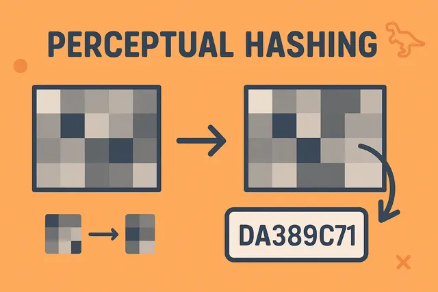
Most perceptual hashing algorithms follow a similar pattern:
- Reduce Size - Shrink image to remove high-frequency details
- Simplify Colors - Convert to grayscale to focus on structure
- Transform - Apply mathematical transformation (often DCT)
- Extract Features - Keep only the most significant information
- Generate Hash - Convert features to a binary fingerprint
The magic is in choosing transformations that preserve perceptually important features while discarding noise.
Real-World Applications
Before diving into the implementation, let’s see where perceptual hashing is used:
- Duplicate Detection - Finding re-posts on social media
- Copyright Protection - Identifying unauthorized use of images
- Content Moderation - Blocking previously flagged inappropriate content
- Similar Image Search - “Find images like this one”
- Video Deduplication - Detecting re-uploaded videos with minor edits
Building pHash from Scratch
Let’s implement a popular perceptual hashing algorithm called pHash. We’ll start simple and gradually add sophistication.
Step 1: Define the Foundation
First, let’s establish our types and basic structure:
// Core types for our perceptual hash implementation
interface ImageData {
  width: number;
  height: number;
  data: Uint8Array; // RGBA pixel data
}

interface PHashConfig {
  hashSize?: number;      // Size of the hash in bits (default: 64)
  imageSize?: number;     // Size to resize image before hashing (default: 32)
  highFreqFactor?: number; // Factor for DCT coefficient selection (default: 4)
}

// Result of hashing includes the hash and intermediate steps for visualization
interface PHashResult {
  hash: bigint;           // The actual hash value
  hashBits: string;       // Binary string representation
  // Debug info for understanding the algorithm
  debug?: {
    resized: number[][];     // Resized grayscale image
    dct: number[][];        // DCT coefficients
    median: number;         // Median DCT value
  };
}

// Main function signature
function perceptualHash(
  image: ImageData,
  config: PHashConfig = {}
): PHashResult {
  const { hashSize = 64, highFreqFactor = 4 } = config;
  // We'll build this step by step
  return {
    hash: 0n,
    hashBits: ''
  };
}
Step 2: Image Preprocessing
The first step is reducing the image to its essential structure. We resize it to a small square to remove fine details:
// Convert RGBA image data to grayscale
function toGrayscale(image: ImageData): number[][] {
  const { width, height, data } = image;
  const grayscale: number[][] = [];

  for (let y = 0; y < height; y++) {
    const row: number[] = [];
    for (let x = 0; x < width; x++) {
      const idx = (y * width + x) * 4;
      // Standard grayscale conversion weights
      const gray = 0.299 * data[idx] +     // Red
                   0.587 * data[idx + 1] +  // Green
                   0.114 * data[idx + 2];   // Blue
      row.push(gray);
    }
    grayscale.push(row);
  }

  return grayscale;
}

// Resize image using bilinear interpolation
function resizeImage(
  pixels: number[][],
  newWidth: number,
  newHeight: number
): number[][] {
  const oldHeight = pixels.length;
  const oldWidth = pixels[0].length;
  const resized: number[][] = [];

  // Calculate scaling factors
  const xRatio = oldWidth / newWidth;
  const yRatio = oldHeight / newHeight;

  for (let y = 0; y < newHeight; y++) {
    const row: number[] = [];
    for (let x = 0; x < newWidth; x++) {
      // Map to original image coordinates
      const srcX = x * xRatio;
      const srcY = y * yRatio;

      // Get the four surrounding pixels
      const x0 = Math.floor(srcX);
      const x1 = Math.min(x0 + 1, oldWidth - 1);
      const y0 = Math.floor(srcY);
      const y1 = Math.min(y0 + 1, oldHeight - 1);

      // Calculate interpolation weights
      const wx = srcX - x0;
      const wy = srcY - y0;

      // Bilinear interpolation
      const value = (1 - wx) * (1 - wy) * pixels[y0][x0] +
                    wx * (1 - wy) * pixels[y0][x1] +
                    (1 - wx) * wy * pixels[y1][x0] +
                    wx * wy * pixels[y1][x1];

      row.push(value);
    }
    resized.push(row);
  }

  return resized;
}
Step 3: The Heart of pHash - Discrete Cosine Transform
The DCT is what makes pHash robust. It transforms the image into frequency space, where low frequencies represent structure and high frequencies represent details:
// 2D Discrete Cosine Transform Type II
function dct2d(matrix: number[][]): number[][] {
  const size = matrix.length;
  const result: number[][] = Array(size).fill(null)
    .map(() => Array(size).fill(0));

  // DCT formula constants
  const c0 = 1 / Math.sqrt(size);
  const c1 = Math.sqrt(2 / size);

  for (let u = 0; u < size; u++) {
    for (let v = 0; v < size; v++) {
      let sum = 0;

      // Sum over all pixels
      for (let x = 0; x < size; x++) {
        for (let y = 0; y < size; y++) {
          sum += matrix[y][x] *
                 Math.cos(((2 * x + 1) * u * Math.PI) / (2 * size)) *
                 Math.cos(((2 * y + 1) * v * Math.PI) / (2 * size));
        }
      }

      // Apply normalization factors
      const cu = u === 0 ? c0 : c1;
      const cv = v === 0 ? c0 : c1;
      result[v][u] = cu * cv * sum;
    }
  }

  return result;
}

// Extract low-frequency DCT coefficients (top-left corner)
function extractLowFrequencies(dct: number[][], size: number): number[] {
  const coefficients: number[] = [];

  // Take top-left corner, excluding DC component (0,0)
  for (let y = 0; y < size; y++) {
    for (let x = 0; x < size; x++) {
      if (x === 0 && y === 0) continue; // Skip DC component
      coefficients.push(dct[y][x]);
    }
  }

  return coefficients;
}
Step 4: Generate the Binary Hash
Now we convert the DCT coefficients into a binary hash by comparing each to the median:
// Calculate median of an array
function calculateMedian(values: number[]): number {
  const sorted = [...values].sort((a, b) => a - b);
  const mid = Math.floor(sorted.length / 2);

  if (sorted.length % 2 === 0) {
    return (sorted[mid - 1] + sorted[mid]) / 2;
  }
  return sorted[mid];
}

// Convert DCT coefficients to binary hash
function generateHash(coefficients: number[]): bigint {
  const median = calculateMedian(coefficients);
  let hash = 0n;

  // Each coefficient becomes one bit
  for (let i = 0; i < coefficients.length; i++) {
    if (coefficients[i] > median) {
      // Set bit i to 1
      hash |= (1n << BigInt(i));
    }
  }

  return hash;
}

// Convert hash to binary string for visualization
function hashToBinaryString(hash: bigint, bits: number): string {
  return hash.toString(2).padStart(bits, '0');
}
Step 5: Complete Implementation
Let’s put it all together:
function perceptualHash(
  image: ImageData,
  config: PHashConfig = {}
): PHashResult {
  const {
    hashSize = 64,
    imageSize = 32,
    highFreqFactor = 4
  } = config;

  // Calculate DCT size needed for desired hash size
  const dctSize = Math.ceil(Math.sqrt(hashSize)) + 1;

  // Step 1: Convert to grayscale
  const grayscale = toGrayscale(image);

  // Step 2: Resize to small square
  const resized = resizeImage(grayscale, imageSize, imageSize);

  // Step 3: Apply DCT
  const dct = dct2d(resized);

  // Step 4: Extract low frequencies
  const coefficients = extractLowFrequencies(dct, dctSize);

  // Step 5: Generate hash
  const hash = generateHash(coefficients.slice(0, hashSize));
  const hashBits = hashToBinaryString(hash, hashSize);

  return {
    hash,
    hashBits,
    debug: {
      resized,
      dct,
      median: calculateMedian(coefficients)
    }
  };
}
Step 6: Comparing Hashes
The beauty of perceptual hashes is how we compare them. We use Hamming distance - counting bits that differ:
// Calculate Hamming distance between two hashes
function hammingDistance(hash1: bigint, hash2: bigint): number {
  // XOR shows bits that differ
  let xor = hash1 ^ hash2;
  let distance = 0;

  // Count set bits (Brian Kernighan's algorithm)
  while (xor !== 0n) {
    xor &= xor - 1n;
    distance++;
  }

  return distance;
}

// Calculate similarity percentage
function calculateSimilarity(
  hash1: bigint,
  hash2: bigint,
  hashSize: number = 64
): number {
  const distance = hammingDistance(hash1, hash2);
  return ((hashSize - distance) / hashSize) * 100;
}

// Determine if images are similar based on threshold
function areSimilar(
  hash1: bigint,
  hash2: bigint,
  threshold: number = 5
): boolean {
  return hammingDistance(hash1, hash2) <= threshold;
}
Advanced Techniques
Our implementation covers the basics, but production systems often include:
Rotation Invariance
To handle rotated images, compute hashes for multiple rotations:
function rotationInvariantHash(image: ImageData): bigint[] {
  const hashes: bigint[] = [];

  // Generate hashes for 0°, 90°, 180°, 270°
  for (let rotation = 0; rotation < 360; rotation += 90) {
    const rotated = rotateImage(image, rotation);
    const result = perceptualHash(rotated);
    hashes.push(result.hash);
  }

  return hashes;
}
Radial Hash Projection
For even better rotation invariance, use radial projections:
function radialHash(image: ImageData): bigint {
  // Convert to polar coordinates
  const polar = cartesianToPolar(image);

  // Apply 1D DCT to radial projections
  const projections = computeRadialProjections(polar);

  // Generate hash from projections
  return generateRadialHash(projections);
}
Multi-Resolution Hashing
Combine hashes at different scales for better accuracy:
function multiResolutionHash(image: ImageData): bigint[] {
  const scales = [16, 32, 64];
  return scales.map(size => {
    const config = { imageSize: size };
    return perceptualHash(image, config).hash;
  });
}
Performance Considerations
For production use, consider these optimizations:
- SIMD Instructions - Use WebAssembly SIMD for faster DCT
- GPU Acceleration - Compute multiple hashes in parallel
- Approximate DCT - Trade accuracy for speed with faster transforms
- Cached Preprocessing - Store resized versions for common sizes
Practical Usage Example
Here’s how you might use perceptual hashing in a real application:
class ImageDatabase {
  private hashes = new Map<string, bigint>();

  addImage(id: string, image: ImageData): void {
    const { hash } = perceptualHash(image);
    this.hashes.set(id, hash);
  }

  findSimilar(image: ImageData, threshold: number = 5): string[] {
    const { hash: queryHash } = perceptualHash(image);
    const similar: string[] = [];

    for (const [id, hash] of this.hashes) {
      if (hammingDistance(queryHash, hash) <= threshold) {
        similar.push(id);
      }
    }

    return similar;
  }
  detectDuplicate(image: ImageData): boolean {
    return this.findSimilar(image, 3).length > 0;
  }
}
Summary
Perceptual hashing creates robust visual fingerprints that survive common image modifications. By combining image preprocessing, frequency transforms, and binary encoding, we can reduce megabytes of image data to just 8 bytes while preserving visual similarity.
Key takeaways:
- Use DCT to extract frequency information
- Low frequencies capture structure, high frequencies capture noise
- Hamming distance efficiently measures hash similarity
- Small implementation (~200 lines) with powerful applications
Whether you’re building a photo sharing platform, copyright detection system, or content moderation tool, perceptual hashing provides an elegant solution for image similarity at scale.